Getting Started
For an easy start with the Python Interface, install divERGe from pip via
pip install diverge-flow
You find a tutorial for the C interface here. You can further download divERGe.tar.gz to obtain a pre-compiled copy of divERGe that additionally contains the C Interface and some Examples. For more pre-built versions, see releases. If you wish to compile yourself to include various optimizations (MPI, CUDA, …), you can do so by cloning the git repository and following the build instructions. Moreover, environment variables can be used to change the number of threads for different components, see Runtime Tuning.
Usage
The C Interface represents the centrum of divERGe. Python specific library features (e.g. the Autoflow function) are documented here. For reading the output files, see the documentation for diverge.output and also the Python doc obtained from within Python using help(object), i.e.,
import diverge.output as do
help(do.diverge_model)
help(do.diverge_post_tu)
In general, the naming for Python functions follows the C function naming,
except for that the diverge_ prefix is omitted.
We now continue with the example: On a not-too-old Linux machine (GLIBC >= 2.17), extract the tar.gz file and use a python3 interpreter to execute the simple example.
mkdir divERGe
tar -C divERGe -xvf divERGe.tar.gz
cd divERGe
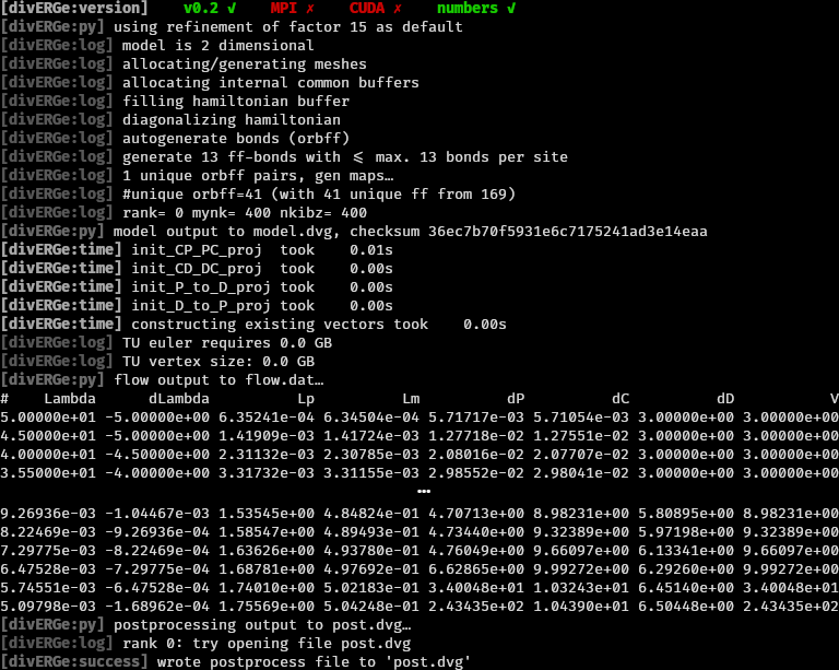
You should now see output as below:
Troubleshooting
If the pip installation fails, you can navigate to the folder where you extracted diverge.tar.gz and execute
python3 setup.py install
Congratulations
You’ve just managed to do your first FRG simulation of a square lattice Hubbard model that displays \(d\)-wave superconductivity! Now let’s take a look at the output:
Besides the compilation status of the library (first line) and some logging
information (prefixed with [divERGe:logname]), the on-line output contains
information on chosen defaults and other miscellaneous information (prefixed
with #): We observe that two files have been written: model.dvg (containing
everything set in the Model) and post.dvg (see Postprocessing and Output). To read the .dvg files, we strongly suggest to use the function
provided in the python library (see Simulation Output). Apart from the
output files, the values for the scale and integration of the flow equations as
table with entries Lambda, dLambda, Lp, Lm, dP, dC, dD, V are printed This
output can be conveniently piped to a file to obtain a flow data file for
further processing. Instead of
python3 examples/simple.py
you can call
python3 examples/simple.py > flow.dat
to obtain three files as output: model.dvg, post.dvg, and flow.dat (with the flow information). The columns in flow.dat correspond to:
- Lambda:
the current scale
- dLambda:
the step size
- Lp:
the particle particle loop maximum
- Lm:
the particle hole loop maximum
- dP:
the differential (for grid and patch) or absolute (for tu) channel maximum in the particle particle channel
- dC:
the differential (for grid and patch) or absolute (for tu) channel maximum in the crossed particle hole channel
- dD:
the differential (for grid and patch) or absolute (for tu) channel maximum in the direct particle hole channel
- V:
the absolute maximum element of the vertex (for grid/patch) or maximum of the channel maxima (tu)
License
divERGe is published under the GPLv3. The license is found in the
git repo. License information from within divERGe
can be obtained by calling diverge_license() or
diverge_license_print().